This blog post describes the process of staging data in Google Cloud Storage and then mapping this to Google BigQuery to provide a low-cost SQL interface for Big Data analysis. There is an R package for connecting to Google Big Query, called bigrquerythat can be used to connect to Google BigQuery and interface with it directly from R-Studio. Some simple examples of combining the power of SQL in BigQuery with R analysis and the Google Mapping API are provided at the end of the blog.
Although the Google BigQuery service is chargeable, it provides a very cost-effective way of working with larger data-sets compared to standing up a traditional relational database server or Hadoop solution.
This blog takes the approach of using the Google Cloud command-line tools (bundled with the Google Cloud SDK) instead of using the GUI web-portal or API calls.
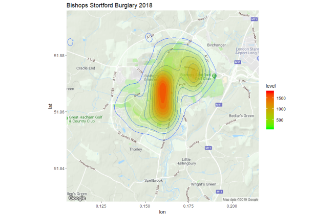
The final section demonstrates using the R ggmap utility for the Google Maps API to plot crime-density maps using the data staged to BigQuery such as the following example:
Although I just wrote this blog to experiment and familiarise myself with the tools, I got some interesting insight into crime distributions for my home-town which are not as clearly identified with other public data sources and police crime-mapping services, as noted briefly at the end of the post.
1. Stage Some Data in Google Cloud Storage
Google Cloud allows large amounts of data to be stored in Google Cloud storage at relatively low cost. Multiple options are available, but the approach demonstrated in this blog focuses on standard Regional Storage Buckets.
The details of this will change over time and are summarised here: https://cloud.google.com/storage/pricing#storage-pricing
My chosen data-set is the UK Crime data from https://data.police.uk/
To stage the data into Google Cloud, first of all you need to sign up for a Google Cloud account (free for the first 12 months, but you still need to supply your credit card details).
Next, install the Google Cloud SDK on the workstation where you are going to initiate the data transfer from (this could be your laptop). I used a free Google cloud “micro-instance” (a free compute VM, class “f1-micro” with 1 vCPU and 0.6 GB memory) to run the data-transfer into Google cloud storage so that I didn’t have to transfer data over my local home WiFi network to-and-fro between my laptop and the Google cloud.
First, if necessary authorise the SDK to access your cloud account:
gcloud auth login
Unless you already have one, you need to create a Google cloud project to map resources associated with cost allocation and also access control. Use the Google Cloud Web-Console to create the project – this will generate a project-ID for your project name.
Then, use gsutil to create a storage bucket in your project:
gsutil mb -c regional -p my_project_id -l us-central1 gs://my_bucket_name
NOTE:
- The Project ID is the Google Cloud Project ID that you are creating this set of cloud resources in and is different to (but directly related to) the Google Cloud Project Name.
- The URL for storage bucket needs to be unique in the world, so you need to come up with an appropriate naming scheme for your bucket.
- The region needs to be
us-central1for US located BigQuery deployments oreurope-west1for European BigQuery deployments. Other regions (such as us-east1) will not work as an external table data-source for BigQuery (see https://issuetracker.google.com/issues/76127552). - Data can now be copied into this bucket using a file-transfer / copy approach. It is possible to specify folders in the file URL reference to simulate a classic file-system directory structure.
Example – copy a test-file to Google Cloud Storage:
gsutil cp testfile gs:/my_bucket_name//testdata
(this assumes you have created a “testfile” in advance).
We can list files stored in cloud buckets as follows:
gsutil ls gs://my_bucket_name
Copy UK Crime Data to Google Cloud Bucket
There is an API to download UK Crime Data from https://data.police.uk/data/ in JSON format, but instead I chose a very simple approach of just downloading zipped CSV’s from the site. This is a five-step manual process for each date-range set of data:
- On a laptop / PC: Go to the data.police.uk/data web-site and prepare a download file: In the interactive web-page, select all forces and a date-range for a full year of data (or however much you want to download).
- On a laptop / PC: Click the Generate File button at the bottom of the screen then right-click on the Download Now button; copy the link to the URL for this button. We will use this URL to
wgetour data to the cloud VM staging host. - On a Linux VM running in Google Cloud: wget the download link we created previously; EG:
wget https://policeuk-data.s3.amazonaws.com/download/a4a9fa057fa8ba69dff5a60d6f1dd29aced02a32.zip - Unzip the file (the format of the zip file means we can’t process this efficiently in a UNIX pipe through a wget| gunzip | copy process)
- Copy the data to our Google Cloud Storage Bucket:
gsutil cp -r 2018* gs://my_bucket_nameto recursively copy all the unzipped crime data where 2018* is the year string-match for the year we are copying. - Delete the staged data (to free up space) and repeat for another date-range selection.
Using a combination of this process and by downloading older data-sets from https://data.police.uk/data/archive/ eventually I ended up with about 16 GB of UK crime data staged covering 7 years of street-crimes for the UK located in the Google Storage Bucket.
Obviously you don’t need to use a cloud storage platform for this amount of data – this was just a learning exercise. However, the whole exercise described in this blog cost me less than $1 USD.
Google Storage File-Names and File-Paths
Google storage buckets allow you to use slashes (/) in file-names to help logically break up their name-space, however, there is no concept of directories or folders in Google – in reality there is just a bunch of files in a bucket of storage allocation.
The Google tools and interfaces that are used with Google storage have rules and logic built into them to simulate a traditional filesystem behavior which gives the illusion of a filesystem in most situations.
More details on the implementation can be found here: https://cloud.google.com/storage/docs/gsutil/addlhelp/HowSubdirectoriesWork
The practical implication of this is that if we try listing crime-data CSVs with gsutil ls as follows:
gsutil ls -r gs://my_bucket_name/*street.csv
then no files are returned.
However, in our BigQuery table definition file, we can map to all street crime CSV files (for all year-month folders, all locations) as follows:
...
...
"sourceUris": [ "gs://my_bucket_name/*street.csv" ]
...
...
as shown in the next section.
2. Process Data with Google BigQuery
Data that is processed by BigQuery is organised in datasets. This maps the physical location of the data to a logical grouping of data-resources to be processed in BigQuery. Google BigQuery can access data stored in the following formats:
- External Sources: data stored in Google Cloud Storage buckets, Google Cloud BigTable or Google Drive can be mapped and directly queried in BigQuery
- Native Storage: BigQuery datasets created using the BigQuery API or command-line.
There is a performance overhead working directly with External Sources and External Sources can only be used for read-only operations, so typically data is loaded from External Sources into native Big Query dataset storage for further processing.
Map External Table to Google Storage Bucket Data
Full details about using external storage with BigQuery are located here: https://cloud.google.com/bigquery/external-data-cloud-storage
Use the Google Storage URI to refer to the data-location when creating the BigQuery external table. For the UK Crime Data that was staged earlier we need to create a template Table Definition File with contents as shown below to specify the path to the input data. Include "skipLeadingRows": 1 to cater for the header in the CSV files and also set a wild-card path to filter out CSV files that don’t cover street-level crime statistics:
{
"autodetect": true,
"csvOptions": {
"encoding": "UTF-8",
"quote": "\"",
"skipLeadingRows": 1
},
"sourceFormat": "CSV",
"sourceUris": [
"gs://my_bucket_name/*street.csv"
]
}
For the examples in this blog-post, this table definition file is saved as file /tmp/table_def
The autodetect option automatically detects the table schema definition (including row-names and data-types). This can be manually specified at the command-line if necessary (refer to the Google cloud documentation for details).
Create the BigQuery dataset for the table to be defined in:
bq --location="US" mk --dataset --default_table_expiration 157788000 ukcrime
This creates a BigQuery dataset called ukcrime.
Note the location specification – for US and Europe, don’t specify the details of an east / west region – just US or EU. Create the dataset in the same geographic location as the storage on which the data is staged. Make sure to specify the appropriate Project ID (this should match the project-id for the Bucket where data is staged).
The default_table_expiration is specified in seconds – after this duration the data will be auto-deleted.
Create the external table definition:
bq mk --project_id=my_project_id --external_table_definition=/tmp/table_def ukcrime.street_crime
This creates a BigQuery table called street_crime located in the dataset ukcrime.
Removing the Data Table and DataSet Definition
When the table is no longer required, the table and its underlying dataset can be removed as follows:
1. Remove the Table
bq rm --project_id=my_project_id ukcrime.street_crime
2. Remove the DataSet
bq --location="US" rm --dataset my_project_id:ukcrime
Basic Analysis with SQL
Test the ability to query the external data-set by performing a select count(*) with the BigQuery console at https://console.cloud.google.com/bigquery (locate the correct Project-ID, DataSet and Data Table to query) and then execute
SELECT count(*) FROM `project_id.dataset.table_name`
to scan the full external-table data-set – EG:
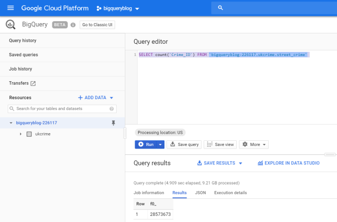
This checks where the data in the CSV files is correctly mapped to the table definition.
BigQuery Command-Line Interface
Details of the BigQuery command line tool bq are located at https://cloud.google.com/bigquery/docs/bq-command-line-tool.
You can set default values for command-line flags by including them in the command-line tool’s configuration file .bigqueryrc
This allows you to set defaults for options such as:
- Geographic location
maximum_bytes_billed(important as this is how BigQuery is charged for and we could potentially query a lot of data)
Set a default Project ID to avoid specifying it for each query as follows:
gcloud config set project
select count(*) from Command Line:
bq query --nouse_legacy_sql 'select count(*) from `my_project_id:my_dataset.table_name`'
Show Details about Data-Set:
bq show my_project_id:my_dataset
Show Details about Table:
bq show my_project_id:ukcrime.street_crime
   Last modified                 Schema                  Type     Total URIs     Expiration      Labels
 ----------------- ---------------------------------- ---------- ------------ ----------------- --------
  01 Jan 15:31:56   |- Crime_ID: string                EXTERNAL   1            01 Jan 21:31:54
                    |- Month: string
                    |- Reported_by: string
                    |- Falls_within: string
                    |- Longitude: float
                    |- Latitude: float
                    |- Location: string
                    |- LSOA_code: string
                    |- LSOA_name: string
                    |- Crime_type: string
                    |- Last_outcome_category: string
                    |- Context: string
First 5 Records
bq query --nouse_legacy_sql 'select * from `my_project_id:ukcrime.street_crime` limit 5'
-+-----------+-------------------+-----------------------+-----------------------+---------+
| Crime_ID |  Month  |       Reported_by        |       Falls_within       | Longitude | Latitude |               Location                | LSOA_code |     LSOA_name     |      Crime_type       | Last_outcome_category | Context |
+----------+---------+--------------------------+--------------------------+-----------+----------+---------------------------------------+-----------+-------------------+-----------------------+-----------------------+---------+
| NULL     | 2010-12 | British Transport Police | British Transport Police | -0.271604 |  50.8344 | On or near Shoreham By Sea            | E01031365 | Adur 002D         | Vehicle crime         | NULL                  | NULL    |
| NULL     | 2010-12 | British Transport Police | British Transport Police |  -3.55944 |  54.6445 | On or near Workington                 | E01019121 | Allerdale 009E    | Violent crime         | NULL                  | NULL    |
| NULL     | 2010-12 | British Transport Police | British Transport Police |  -3.55944 |  54.6445 | On or near Workington                 | E01019121 | Allerdale 009E    | Violent crime         | NULL                  | NULL    |
| NULL     | 2010-12 | British Transport Police | British Transport Police |  -1.36974 |  53.1007 | On or near Alfreton                   | E01019400 | Amber Valley 001A | Violent crime         | NULL                  | NULL    |
| NULL     | 2010-12 | British Transport Police | British Transport Police |  -1.36974 |  53.1007 | On or near Alfreton                   | E01019400 | Amber Valley 001A | Violent crime         | NULL                  | NULL    |
Select Group-By Operation (1):
bq query --nouse_legacy_sql 'select `Reported_by`, count(*) from `my_project_id.ukcrime.street_crime` group by `Reported_by` '
+------------------------------------+---------+
|            Reported_by             |   f0_   |
+------------------------------------+---------+
| South Yorkshire Police             | 1506929 |
| West Mercia Police                 |  948811 |
| South Wales Police                 | 1081292 |
| Leicestershire Police              |  699633 |
| Surrey Police                      |  733160 |
| Gloucestershire Constabulary       |  448755 |
| Police Service of Northern Ireland | 1147169 |
| West Midlands Police               | 2125849 |
| Nottinghamshire Police             |  934659 |
| Suffolk Constabulary               |  513281 |
| British Transport Police           |  379333 |
| Kent Police                        | 1388975 |
| North Yorkshire Police             |  556991 |
| Cheshire Constabulary              |  725226 |
| Devon & Cornwall Police            | 1078448 |
| Greater Manchester Police          | 2778117 |
| West Yorkshire Police              | 2247592 |
| NULL                               |   48085 |
| Humberside Police                  |  740223 |
| Merseyside Police                  | 1241501 |
| Wiltshire Police                   |  454743 |
| Metropolitan Police Service        | 8256277 |
| Staffordshire Police               |  816209 |
| Essex Police                       | 1318168 |
| Sussex Police                      | 1182637 |
| Warwickshire Police                |  405568 |
| Norfolk Constabulary               |  574457 |
| Cambridgeshire Constabulary        |  611133 |
| Thames Valley Police               | 1398430 |
| Derbyshire Constabulary            |  801798 |
| Cumbria Constabulary               |  359497 |
| Avon and Somerset Constabulary     | 1341566 |
| Durham Constabulary                |  540664 |
| Dyfed-Powys Police                 |  320767 |
| Hertfordshire Constabulary         |  778193 |
| Lincolnshire Police                |  490573 |
| Bedfordshire Police                |  513544 |
| Hampshire Constabulary             | 1449141 |
| Lancashire Constabulary            | 1475558 |
| Northamptonshire Police            |  633954 |
| Northumbria Police                 | 1345206 |
| Cleveland Police                   |  709250 |
| Dorset Police                      |  562290 |
| Gwent Police                       |  498521 |
| City of London Police              |   56255 |
| North Wales Police                 |  507564 |
+------------------------------------+---------+
Select Group-By Operation (2):
bq query --nouse_legacy_sql 'select `Crime_type`, count(*) from `my_project_id.ukcrime.street_crime` group by `Crime_type`'
+------------------------------+----------+
|          Crime_type          |   f0_    |
+------------------------------+----------+
| Public disorder and weapons  |   242145 |
| Other theft                  |  4101195 |
| Violence and sexual offences |  6601077 |
| Shoplifting                  |  2471591 |
| Bicycle theft                |   532959 |
| Burglary                     |  3523358 |
| Public order                 |  1434310 |
| Possession of weapons        |   170662 |
| Violent crime                |  1673219 |
| Theft from the person        |   501794 |
| Vehicle crime                |  3176375 |
| Criminal damage and arson    |  4035402 |
| Other crime                  |  2298189 |
| Robbery                      |   511750 |
| Anti-social behaviour        | 16249075 |
| Drugs                        |  1202891 |
+------------------------------+----------+
Copy External Table into Big Query Table
Although we can continue to use the external table as a data-source, we can also use it as a source to create a native BigQuery table that is not staged on regular cloud storage. This has the advantage of being:
- Faster (better performance)
- Support for Update / Insert / Delete rows of data.
- Potentially cheaper for small data-sets (first 10 GB of storage are free and query charges up to 1 TB are free)
The charges for BigQuery data storage and access are listed here: https://cloud.google.com/bigquery/pricing#queries
Follow the instructions here: https://cloud.google.com/bigquery/docs/tables to create a new BigQuery table that has a structure / schema based on the External Table street_crime that we created earlier. In this example, the new table is street_crime_bq:
bq --location=US query --destination_table bigqueryblog-226117:ukcrime.street_crime_bq --use_legacy_sql=false 'SELECT * from `bigqueryblog-226117:ukcrime.street_crime`'
Next, view the size of this table:
bq show  bigqueryblog-226117:ukcrime.street_crime_bq
Table bigqueryblog-226117:ukcrime.street_crime_bq

   Last modified                 Schema                Total Rows   Total Bytes     Expiration      Time Partitioning   Labels
 ----------------- ---------------------------------- ------------ ------------- ----------------- ------------------- --------
  08 Jan 09:16:12   |- Crime_ID: string                48725992     9948025396    08 Jan 15:16:12
                    |- Month: string
                    |- Reported_by: string
                    |- Falls_within: string
                    |- Longitude: float
                    |- Latitude: float
                    |- Location: string
                    |- LSOA_code: string
                    |- LSOA_name: string
                    |- Crime_type: string
                    |- Last_outcome_category: string
                    |- Context: string
Conveniently this is just under 10 GB, so hopefully storage of this will be free under the Google Cloud usage terms.
To free up space (and avoid paying for storage), delete the old external table street_crime and delete the files from the underlying storage bucket:
bq rm -f -t ukcrime.street_crime
gsutil rm -r gs://[my_storage_bucket]/*
3. Connect to BigQuery with R
There is a good introductory tutorial on using R with BigQuery here: https://cloud.google.com/blog/products/gcp/google-cloud-platform-for-data-scientists-using-r-with-google-bigquery
To interact with Google BigQuery from an R session we can use Hadley Wickham’s bigrquery package: https://cran.r-project.org/web/packages/bigrquery/index.html
From within an R session, install the bigrquery package:
R> install.packages("bigrquery")
Next, install the bigrquery development packages (as of the time of writing, there are components we need that are not in a compiled package and need to be installed from source-code):
R> install.packages('devtools')
 devtools::install_github("rstats-db/bigrquery")
Now that BigRQuery is installed and set-up store the Project ID for the dataset that is to be queried in your R session:
R> project = "my_project_id"
Store a SQL query to execute against BigQuery in a string variable:
R> SQL = "SELECT month, count(*)
FROM `[my_project_id]:ukcrime.street_crime_bq`
WHERE Crime_type = 'Burglary'
GROUP BY month"
Then use bq_project_query to run the query, storing the results in an R session variable:
R> results <- bq_project_query(project,SQL)
Running job [\]  6s
Complete
Billed: 1.4 GB
The first time you run a BigQuery request from R, you will be prompted to authorise the session and cache an authrisation token – follow the instructions as shown below, open the Web-URL link provided in a browser, and paste the token back into the R session to save the authorisation:
Use a local file ('.httr-oauth'), to cache OAuth access credentials between R sessions?

1: Yes
2: No

Selection: 1
Adding .httr-oauth to .gitignore
httpuv not installed, defaulting to out-of-band authentication
Enter authorization code: [authorisation_token_from_google-web_auth_screen]
Finally, extract the BigQuery result-set into an R data-frame:
R> burglary <- bq_table_download(results, max_results = 120) Downloading 95 rows in 1 pages. > burglary
# A tibble: 95 x 2
   month     f0_

 1 2011-12 42624
 2 2013-09 36514
 3 2015-06 32413
 4 2013-07 36470
 5 2017-09 36809
 6 2015-08 32551
 7 2014-01 39058
 8 2014-12 36263
 9 2012-04 38184
10 2016-01 35590
# ... with 85 more rows
>
Now that we have our summary result-set locally in the R-session we can do some analysis:
R> burglary$year = substr(burglary$month,1,4)
R> burglary$month = substr(burglary$month,6,7)

R> colnames(burglary)[2] = 'count'

R> ggplot(burglary, aes(fill=year, y=count, x=month)) +
+    geom_bar(position="dodge", stat = "identity")
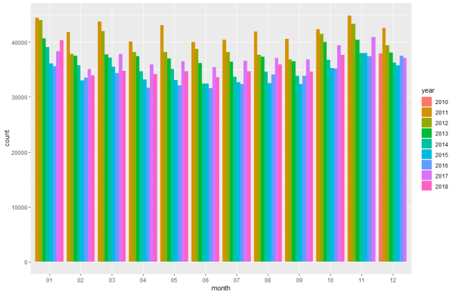
A general overall trend in decreasing burglaries in the UK for the last 8 years can be seen. A quick visual inspection suggests there are some seasonal (monthly) variations, but these don’t look significant. There is an interesting spike in burglaries in 2017 that appears to be falling back a little in 2018.
Mapping Crime Data with ggmap
ggmap Install
The ggmap utility provides access to the Google Maps API. First, install the package – this has to be done from GitHub, not CRAN (details here: https://github.com/dkahle/ggmap ), as we need a more recent version that allows us to interface with the updated Google API:
devtools::install_github("dkahle/ggmap")
Next enable the API. To enable the API go to this link:
https://developers.google.com/maps/documentation/geocoding/get-api-key
and click the “Get Started” button and follow the instructions to enable access to the API for the Google Cloud project (i.e. the [my_project_id] used previously in this blog-post). This creates a Google Maps token that should be copied saved for use later.
Details of charges for using the Maps API can be found here:
https://cloud.google.com/maps-platform/pricing/sheet/
For small volumes of API requests the cost is small to negligible. Ensure that the API token is protected and not checked into code in order to avoid other people using your token and billing their usage to your Google account.
Join to London Crime LSOAs
To map a sub-set of crime-data just for London, it would be useful to a set of LSOA IDs to select from our UK-wide data-set. A list of all London LSOAs can be sourced in the form of a CSV london-lsoa-data.csvfrom this web-URL: https://data.london.gov.uk/dataset/lsoa-atlas
This data can be uploaded to Google Cloud Storage and mapped to a second BigQuery external table called london_lsoa, following the same approach as used for the main crime stats data. Now we have a table we can perform SQL joins against to get a sub-set of London Crime stats.
In R, set a variable to hold the Google Cloud ProjectID in (if not already set) and execute a query against Google BigQuery to return all the Crime Data for a specific month and specific set of LSOAs based on a SQL join condition:
R> library(bigrquery)
R> project = "[my_project_id]"

R> SQL = "SELECT crime.Month, crime.Longitude, crime.Latitude, crime.LSOA_code, crime.LSOA_name, crime.Crime_type
FROM `bigqueryblog-226117.londonlsoa.london_lsoa` as lsoa
JOIN `bigqueryblog-226117.ukcrime.street_crime_bq` as crime
ON lsoa.string_field_0 = crime.LSOA_code
WHERE crime.Month = \"2017-01\" "

R> results <- bq_project_query(project,SQL) Running job [\]  3s Complete Billed: 3.5 GB R> lon_crime <- bq_table_download(results)
Downloading 79,516 rows in 8 pages.
Now, we can load ggmap and try mapping the crime-data.
Mapping crime data
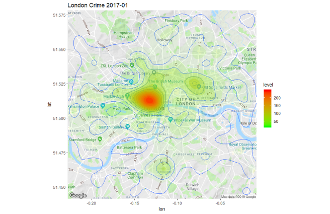
The code below gets a map from Google, centered on some Longitude and Latitude coordinates that we supply, and then plots a density map using geom_density2d to show the areas of the highest crime density. These examples use the data queried earlier that is just for January 2017:
R> library(ggmap)
R> token = '[my_google_api_token]'
R> register_google(token)

#Lon/Lat coords for center of London
R> lat = 51.509865
R> lon = -0.118092

# get a map
R> map = get_map(location = c(lon = lon, lat = lat)
                             , zoom = auto, scale = "auto")
# R> ggmap(map) # plot with no data

#Add some data to a map and plot it
R> p <- ggmap(map, extent = "panel", maprange=FALSE) +
     geom_density2d(data = lon_crime, aes(x=lon_crime$Longitude
                         , y=lon_crime$Latitude)) +
     stat_density2d(data = lon_crime, aes(x=lon_crime$Longitude
                         , y=lon_crime$Latitude
                         , fill = ..level.., alpha = ..level..)
                         , size = 0.01, bins = 16, geom = 'polygon') +
     scale_fill_gradient(low = "green", high = "red") +
     scale_alpha(range = c(0.00, 1.0), guide = FALSE) +
    ggtitle("London Crime 2017-01")
R> print(p)
This produces a plot as shown below:
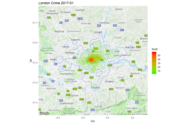 We can see crime is generally centered on the the most densly populated areas of London with a few outliers around Croydon, Romford, Hayes etc. By re-running the
 get_map call with zoom = 12 as follows:
R> map = get_map(location = c(lon = lon, lat = lat)
, zoom = 12, scale = “auto”)
and re-running the code we can zoom in to see more detail in the center of London:
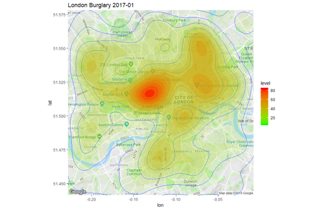
If we change the SQL query against Google Big Query to filter out Burglary Crimes:
SQL = "SELECT crime.Month
  , crime.Longitude
  , crime.Latitude
  , crime.LSOA_code
  , crime.LSOA_name
  , crime.Crime_type
FROM `bigqueryblog-226117.londonlsoa.london_lsoa` as lsoa
JOIN `bigqueryblog-226117.ukcrime.street_crime_bq` as crime
ON lsoa.string_field_0 = crime.LSOA_code
WHERE crime.Month = \"2017-01\"
AND crime.Crime_type = 'Burglary' "
we can see a very different crime distribution, with crimes more evenly distributed across multiple areas of residential housing.
Further experimentation
I used the same approach as above used with a query for a different location (around my home-town of Bishops Stortford) and for a wider time-range (the whole of 2018):
SQL="SELECT crime.Month, crime.Longitude, crime.Latitude, crime.LSOA_code, crime.LSOA_name, crime.Crime_type
FROM `bigqueryblog-226117.ukcrime.street_crime_bq` as crime
WHERE crime.LSOA_name like \"East Hert%\"
AND crime.Month LIKE \"2018%\"
AND crime.Crime_type = 'Burglary' "
and plotted a chart showing burlgary density for 2018. This was quite interesting as it showed that a) my house is outside the danger zone b) burglary is surprisingly focused around the center of town c) there is an interesting burglary hot-spot around the golf-course.